Integrated Gradients for DNA Foundation Models

Introduction

This blog post is for anyone interested in attributive interpretability applied to genomics foundation models, though lessons from this can be extended to other models. We use a method called integrated/expected gradients to find the motifs the model deems most important for transcription factor enhancer activity. This is a long blog post, so you may only be interested in reading some sections. A short guide:

• For those new to the method of integrated gradients, see section Integrated Gradients for the intuition and theory behind the method, and the justification for the method.
• The section Baselines for DNA Models shows which baselines we tested, how model predictions looked at these baselines, and how we tested how many integration steps are needed for ensuring the attributions generated by the baselines satisfy the Completeness Axiom.
• Section Ablation Tests shows how to select the baseline that leads to the attributions that rank the input features in the best order (including how we deal with negative attributions) and which baseline works best for this task and model.
• In Motif Analysis, we describe how we extracted the motifs the model finds most important for transcription factor enhancer activity, show the most important motifs, and match motifs found by the model with known transcription factor binding sites.
• If you are only interested in the main takeaways from this article, see Takeaways.
• The code is available here.

For a sneak peek of the motif matching results, Figure 1 shows some of the motifs the model discovered (left) compared to known, experimentally validated transcription factor binding sites (right) (Ovek Baydar et al., 2026). By applying the expected gradients method carefully, we extracted motifs that match closely with known binding sites, the presence of which drives enhancer activity. This is a critical result confirming that the model, at least in part, anchors its predictions in biological rules.
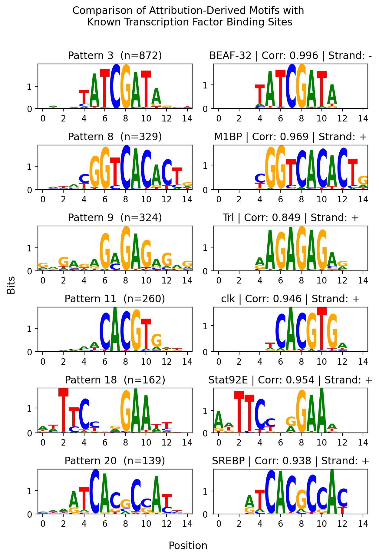Figure 1: Discovered motifs compared to known motifs in JASPAR database (Ovek Baydar et al., 2026).

Summary

Pre-trained foundation models are the state-of-the-art for a wide range of genomics tasks, but extracting useful biological insights from them is complex. One promising method for explaining model predictions with respect to their inputs is integrated gradients, which relies on a “baseline” embedding to compute attribution scores (see this excellent blog post for an in-depth discussion of baselines in image data). However, choosing a good baseline can be tricky because it is often model-specific; a baseline that worked well for one model may not generalise to another. In this article, we show how to create and validate potential baselines using a fine-tuned Nucleotide Transformer v3 on the genomic benchmarking task of predicting gene enhancer activity. The goal is to find the baseline that most effectively explains how the model makes its predictions. We present an end-to-end workflow, from selecting an appropriate baseline through to motif-level biological interpretation, that can serve as a blueprint for interrogating what genomic foundation models have learned.

Background

Machine learning in genomics has shifted from small, specialised models to pre-trained foundation models (Libbrecht and Noble, 2015; Shu et al., 2026). While smaller supervised models offer more transparency, they require extensive annotated data and are limited to specific tasks and organisms. In contrast, genomic foundation models are pre-trained via self-supervision on large, multi-species DNA corpora. These models learn rich, contextual representations and have shown strong performance across different genomics tasks, from variant effect prediction to chromatin accessibility and gene expression (Boshar et al., 2025; InstaDeep, 2026).

However, the vast number of parameters in these foundation models makes it difficult to understand how they generate predictions. This opacity is particularly problematic in biology, where use cases include high-stakes therapeutic and clinical settings. Models might make predictions for incorrect reasons or they may have learned novel biological mechanisms, both of which remain hidden from the practitioner.

This challenge has driven ongoing efforts to develop interpretability methods for foundation models more broadly. One way to approach interpretability is through attribution, which answers the question “How did different parts of the input contribute to a given prediction?” This is the approach we focus on in this article.

There has been previous work on applying interpretability methods to biological foundation models (Anthropic, 2025; Consens et al., 2025), including attribution methods (Majdandzic et al., 2023). However, existing work lacks specific guidelines on how to systematically apply these methods to discrete biological data like DNA sequences. For instance, while the attribution method integrated gradients has been applied to image data extensively, it is less clear how to optimally configure it for biological sequence models to ensure robust and biologically valid results (Sturmfels et al., 2020; Sundararajan et al., 2017; Xu et al., 2020).

In this article, we explore the adaptations needed for applying integrated gradients on DNA sequence data (Sundararajan et al., 2017). We provide an analysis on the choice of baseline, including how to assess its suitability for a particular model and dataset via ablation tests. We demonstrate this using the Nucleotide Transformer v3 model on the task of enhancer activity prediction (Boshar et al., 2025; de Almeida et al., 2022), and further investigate how TF-MoDISco can be incorporated for motif discovery (Shrikumar et al., 2018).

Dataset, Training and Model

Model

As a model, we chose the pre-trained Nucleotide Transformer 3, specifically the smallest 8M parameter variant, so we could easily fine-tune and compute attributions at single nucleotide resolution (Boshar et al., 2025).

When using integrated gradients, we do not input sequences directly into the model, but we feed it embeddings. The embeddings, matrices of shape sequence length by embedding dimension, are how the model represents DNA sequences. Specifically, the model is fed an interpolation between the embedding of some DNA sequence and a so-called baseline embedding. For more details on what this means, see section Integrated Gradients. Figure 2 shows the architecture of the Nucleotide Transformer 3 model, including where the integrated gradients input is inserted (Boshar et al., 2025). 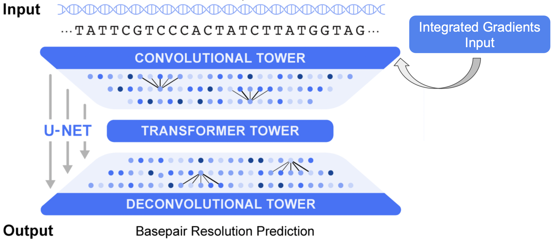Figure 2: Diagram of NTv3 with integrated gradients input. Adapted from Boshar et al., 2025.

Dataset and Training

We fine-tuned NTv3 on the enhancer activity task described in the DeepSTARR paper (de Almeida et al., 2022), which is now a popular benchmarking dataset for DNA foundation models. The dataset quantifies the enhancer activity of 249 base pair (bp) long sequences paired with either one housekeeping or one developmental promoter in Drosophila melanogaster S2 cells. We chose this task due to the explicit correlation between the nucleotide sequence and its corresponding enhancer function as well as the modest computational requirements with short sequences of 249 bp, which allowed for local training and analysis.

We fine-tuned the 8M NTv3 model on the DeepSTARR chromosome training split publicly accessible at https://huggingface.co/datasets/GenerTeam/DeepSTARR-enhancer-activity. See Appendix A for the hyperparameters we used for fine-tuning, which were not extensively tuned.

Fine-tuning leads to performance comparable to DeepSTARR, measured by a Pearson correlation coefficient (PCC) of 0.65 and $R^2$ of 0.46 on the held out test set (Figure 3). The original DeepSTARR CNN model achieved a PCC of 0.68, which is near the upper bound of PCC=0.73 between two technical replicates (de Almeida et al., 2022).
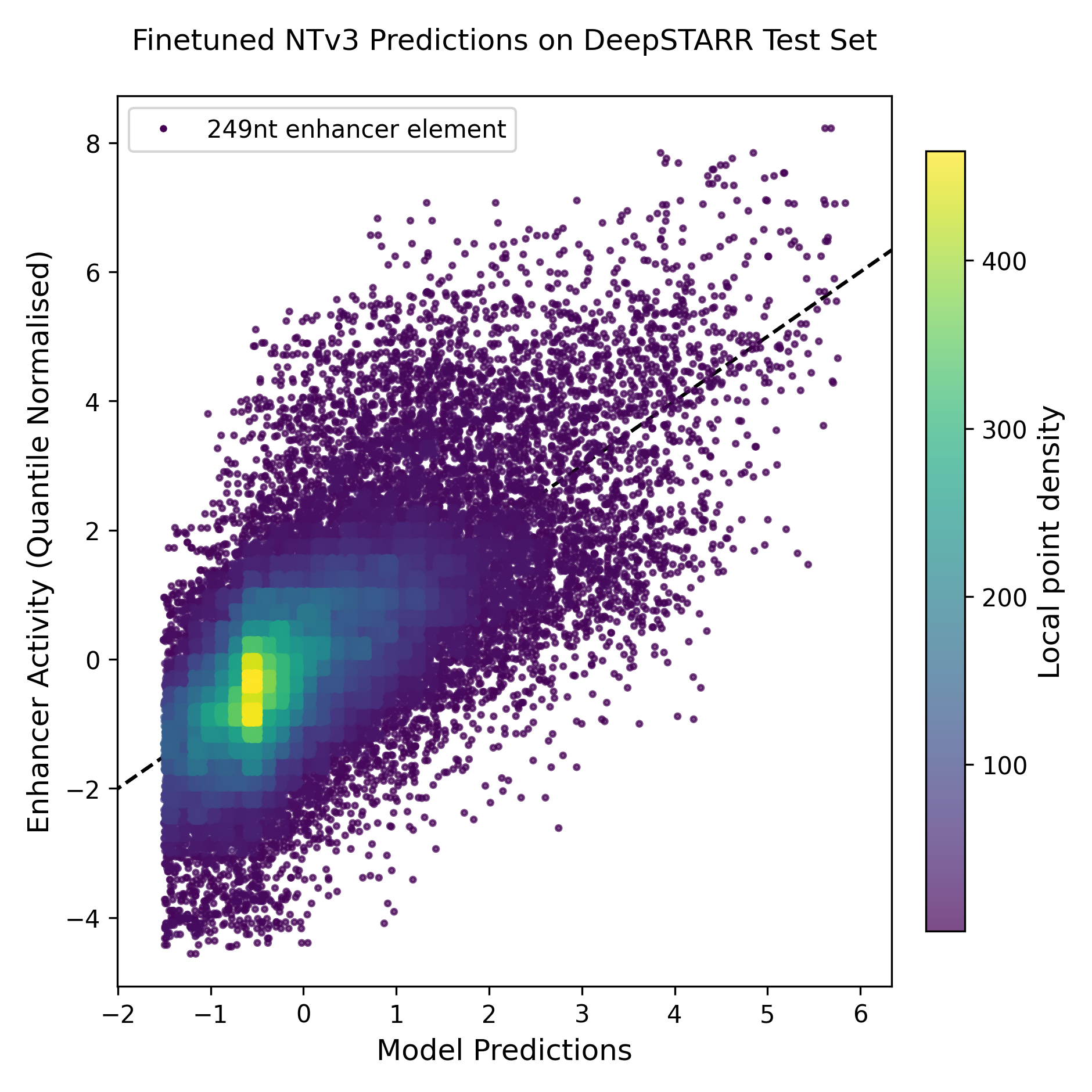Figure 3: NTv3 predictions vs. ground truth enhancer activity.
From the test set, we select a random subset of 200 sequences on which we evaluate the quality of the attributions resulting from different baselines. Having found the baseline resulting in the best attributions on this subset, we use this baseline to find the attributions on the entire test set and extract attribution-enriched motifs from these attributions.

Integrated Gradients

Justification

Saliency maps, an early gradient-based attribution method, work by taking the gradient of the model’s output with respect to its input (Simonyan et al., 2014). To understand the intuition behind this, take the example of image classification. An image is made of pixels, so each pixel is one feature of the model input. The gradient of the model output represents how much a tiny change in a specific input feature would change the output. If this change is large, then this feature must be important. However, the problem is that gradients can saturate: for instance, a dog detection model could be so confident that an image contains a dog that no change in any single feature would lead to a significant change in the model’s prediction, thus leading the saliency map to output that no feature is particularly important. Integrated gradients uses the concept of a baseline to solve this problem.

The baseline is an input to the model that is supposed to represent the absence of any features. Integrated gradients aims to explain the change in model prediction at the input of interest (from now on referred to as the target input) and at the baseline.

Intuition

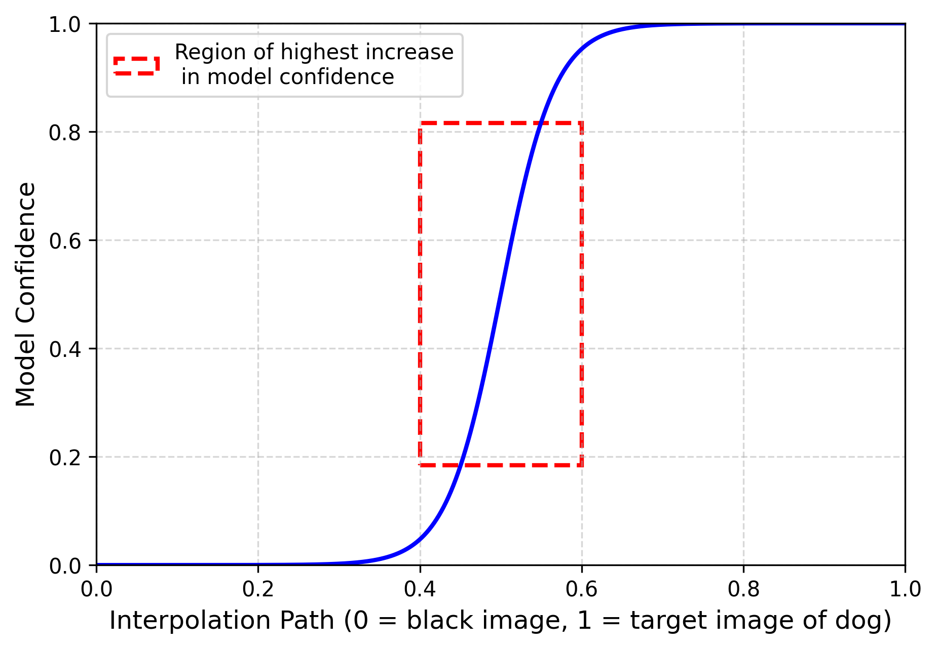Figure 4: Intuition on gradient saturation.
Consider again the example of dog detection. In this case, the baseline could be a fully black image, at which the model should be certain no dog is present in the image. Imagine now interpolating between the baseline and an image containing a golden retriever, the target input, where the model is near 100% certain a dog is in the image. By interpolation, we mean creating a sequence of images that gradually fades in the target image from the pure black image. We can then calculate the gradients for each image in this sequence. In Figure 4 above, the model’s confidence is nearly identical between the 0.8 and 1.0 marks on the interpolation path. This means the gradients at the final image are saturated — altering the pixels slightly has almost no effect on the prediction — so no individual pixel receives a high importance score.

Integrated gradients solves this problem by accumulating the gradients across every image in the sequence: even if the model’s gradients are saturated for the final image, there are earlier points in the sequence where the dog first becomes recognisable; in Figure 4, this occurs midway along the interpolation path between 0.4 and 0.6, denoted by the red rectangle. In those images, the gradients for the pixels making up the dog are large because the model’s prediction is increasing a lot. By accumulating them, we capture the importance of each pixel before the model’s gradients saturate, giving us a good indication of which pixels drive the model’s prediction.

Theory

Formally, integrated gradients is defined as follows (Sundararajan et al., 2017):

\(\begin{equation} \text{IntegratedGrads}_i(x) ::= (x_i - x_i') \times \int_{\alpha=0}^{1} \frac{\partial F(x' + \alpha(x - x'))}{\partial x_i} \, d\alpha \end{equation}\) $F$ is the model, $x$ is the input, $x’$ is the baseline, $i$ is the index of the $i$’th input feature, $\frac{\partial F(x)}{\partial x}$ is the gradient of $F(x)$ in the direction of the $i$’th input feature, and $\alpha$ is the interpolation parameter. The integral is the accumulation of gradients from the baseline to the target input; it calculates the average gradient between the baseline and the target input for feature $i$. We multiply by $(x_i - x_i’)$, the distance between the value of feature $i$ at the target input and at the baseline, to get the total change in the prediction caused by this feature. Beyond the original integrated gradients paper, there are other research papers and blog posts that delve further into the theory and how to use integrated gradients for specific applications (Sturmfels et al., 2020; Xu et al., 2020).

Checking Attribution Validity

The integral needs to be approximated as a sum, requiring a specific number of integration steps. The Completeness Axiom can be used as a practical check if enough integration steps have been used. This axiom states that attributions add up to the difference between the model output at the target input and the baseline, meaning that they explain exactly how much each input feature $i$ contributes to moving the output from the output at the baseline to the output at the target input. Formally:

\(\begin{equation} \sum_{i=1}^{n} \text{IntegratedGrads}_i(x) = F(x) - F(x') \end{equation}\)

Given that we must use numerical integration and that the model function may not be smooth at all points, we need to check whether we have used enough integration steps. We should also check whether we have an appropriate baseline by verifying that the completeness axiom is satisfied.

We define:

\(\begin{equation} \delta = \sum_{i=1}^{n} \text{IntegratedGrads}_i(x) - (F(x) - F(x')) \end{equation}\)

Because the absolute approximation error $\delta$ scales with the magnitude of the model’s output difference $(F(x)−F(x’))$, it cannot be evaluated uniformly across different sequences. Therefore, we use the relative error ratio $\epsilon$ to measure the proportion of the prediction difference unaccounted for by the numerical approximation:

\(\begin{equation} \epsilon = \left| \frac{\delta}{F(x) - F(x')} \right| \end{equation}\)

We consider any sequence with $\epsilon \geq 0.1$ to not have converged sufficiently to be informative.

Expected Gradients

We also use an extension of integrated gradients that relies on choosing baselines from a distribution rather than deterministically, thus minimising the bias introduced by using a single deterministic baseline. Such random baselines can include, for instance, a random DNA sequence (Erion et al., 2020).

\(\begin{equation} \text{ExpectedGrads}_i(x) ::= \mathbb{E}_{x' \sim D,\, \alpha \sim U(0,1)} \left[ (x_i - x'_i) \times \frac{\partial F(x' + \alpha(x - x'))}{\partial x_i} \right] \end{equation}\)

$D$ is the distribution of the baselines. $U$ is the uniform distribution. Expected gradients also satisfies the completeness axiom (Equation 2) (Erion et al., 2020).

A Note on Baseline Choice

At the start of this section, a baseline is described as the “absence” of input features, but this is a challenging concept to define. In a computer vision task, a natural choice of baseline could be all zeros, or a black image. However, if the input image contains a black dog, this would be assigned zero importance (since $x_i - x_i’ = 0$ in Equation 1) irrespective of how relevant it is to the prediction. It is worth noting that baselines do not always need to perfectly represent “missingness” of a feature: Alternative baseline options have been explored in computer vision (Sturmfels et al., 2020), some of which do contain information from the target input. DNA sequence data also has additional considerations, such as the fact that a baseline might not correspond to a valid nucleotide sequence, depending on how embeddings are perturbed. This and other questions are explored in more detail in the next few sections.

Comparison to In-Silico Mutagenesis

There are much simpler ways to approximate the impact of each nucleotide in a DNA sequence on the model output, such as in-silico mutagenesis (ISM). ISM evaluates feature importance by replacing nucleotides in the sequence one by one and measuring the resulting change in the model’s prediction. You may be wondering why one would choose to use integrated gradients when simpler methods like ISM exist.

For long sequences, integrated gradients is more computationally efficient. For a sequence of length $n$, evaluating every possible single-point mutation requires $3n$ separate forward passes, as there are three alternative nucleotides for each position. Conversely, integrated gradients requires a fixed number of forward and backward passes equal to the chosen number of integration steps (in our case, between 200 and 1,000 depending on the baseline). However, for our task with sequence length of 249, ISM requires 747 forward passes, making it computationally comparable to or even cheaper than integrated gradients.

Another justification for using integrated gradients is its ability to capture non-linear interactions between features. Take for example a situation where two motifs in a DNA sequence form a logical OR gate, i.e. removing only one of the motifs does not change the model prediction, only removing both does. Then, mutating a single motif in ISM yields no substantial change in the model output (as it can at most affect one of the motifs), resulting in near-zero attribution for both functional regions. Integrated gradients resolves this by accumulating gradients along a path from a baseline to the input. Because all features transition from the baseline simultaneously, the model’s prediction changes as both motifs become recognisable. Consequently, both motifs receive credit for their contribution to the final prediction.

Baselines for DNA Models

We chose the following baselines for our integrated gradients experiments:

• Zero embedding: An embedding of all zeros. For images, this is perhaps the most intuitive way of representing a lack of information.
• Overall mean embedding: The overall mean embedding is calculated by first averaging the embeddings across the sequence dimension for each individual sequence, and then taking the average of those resulting vectors across the entire training set. This is the average across everything the model has seen during training. This means it could explain which features in an input sequence lead to an increase/decrease in the predicted target variable compared to the average training set embedding.
• Sequence mean embedding: The mean over the sequence dimension of a single sequence. We try this in case the overall mean is too out-of-distribution for the model, as this one would retain more of the characteristics of an individual sequence. This removes all positional information from the embedding.
• Gaussian blurred embedding: Gaussian kernel slid over the target sequence embedding, only in the sequence dimension. We chose a kernel size of 31 and standard deviation of 5. This blurs positional information without removing it entirely.

We used these baselines for expected gradients:

• Gaussian jitter embedding: Gaussian noise added to the sequence embedding with a standard deviation of 1.0. Random noise is another way of representing no information.
• Random sequence embedding: Embedding of a random sequence. We choose a random nucleotide uniformly at each position. This ensures the input is still a valid sequence, and hence more likely to be in-distribution, while being random.
• Shuffled: The embedding of a sequence after shuffling its nucleotides. This removes all positional information from the embedding while retaining information about the distribution of nucleotides within a sequence. It also remains a valid sequence.
• Training subset: The embedding of a random sequence in a subset of the training set. We randomly chose 1000 sequences from the training set for our experiments. This ensures the baseline is always a valid sequence, and so will not be out-of-distribution.

We also tried the per-position mean embedding (the mean calculated by position-wise averaging the embeddings across the training set), but it was almost the same as the overall mean embedding due to the large size of the training set, composition of the vocabulary, and fixed length windows, so we chose not to include it in further analyses.

Baseline Visualisations

Figure 5 shows the embeddings and the associated baselines for the first 100 nucleotides of an arbitrary sequence taken from the test set.

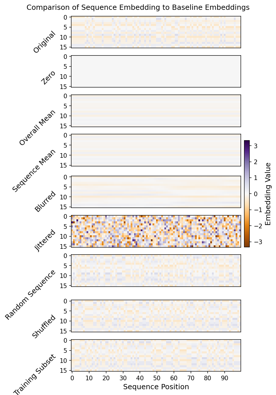Figure 5: Comparison of the embeddings of different baselines. The overall mean and the sequence mean embeddings are very similar, likely because the distribution of nucleotides within this sequence is not far from the one in the training set. The magnitude of the embeddings on the jittered baseline is far greater than the one in the other embeddings, which could raise concerns that it may be too far out-of-distribution for the model to deal with. However, these concerns will be alleviated later on. This shows the embedding values only for one sequence. Figure 6 shows the distributions of the embedding values across the dataset selected for attribution analysis.

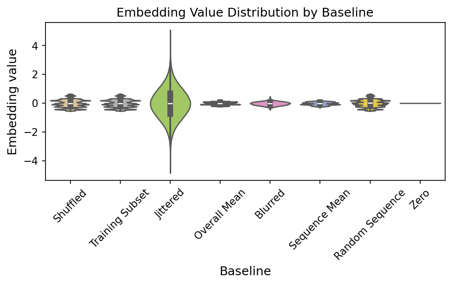Figure 6: Distribution of embedding values by baseline across the attribution dataset.

Note that the distribution of the embedding values for the shuffled baseline is the same as the distribution for the embeddings of the original sequences. The noise introduced by the jittered baseline is so strong that there are many embedding values that are highly out of distribution compared to those of the original sequences.

It is important to know the distribution of the model predictions for each of the baselines because it can strongly bias the attributions. For instance, if the prediction at a baseline is consistently very high compared to the prediction at the target sequences, then at least some nucleotides will have very negative attributions. We visualise the prediction range for each of our baselines in Figure 7:

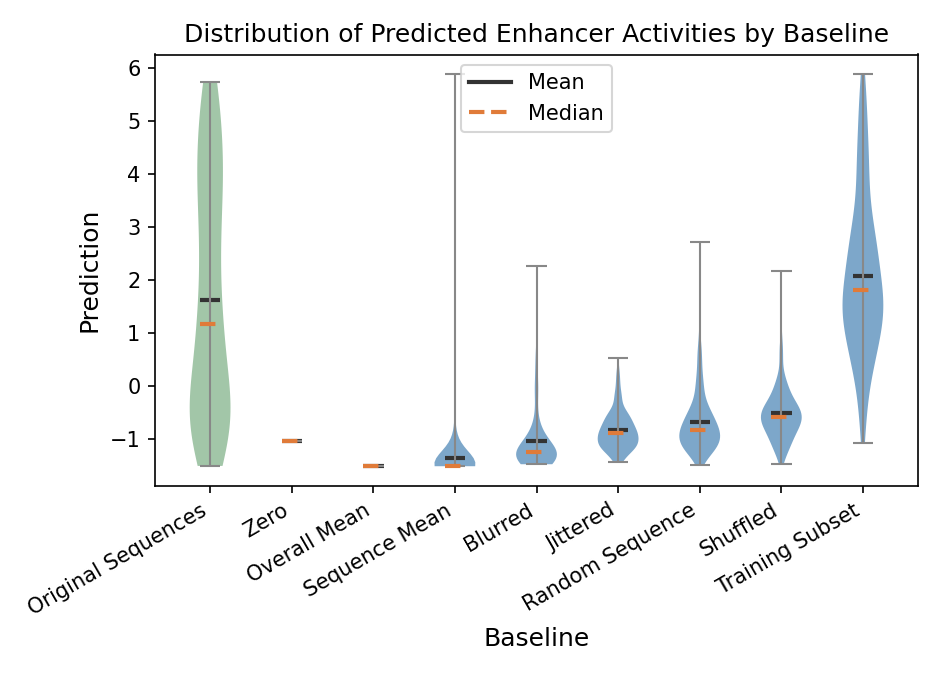Figure 7: Distribution of model predictions at each baseline. Most baselines yield lower predictions than the target sequences.

The average predictions at the baselines are lower than those for the original sequences for all baselines except the training subset baseline. Given this, the attributions for these baselines are likely to be majority positive in order to explain the shift from the lower prediction at the baseline to the higher prediction at the target sequence. Even though the embedding values of the jittered baselines are out of distribution as seen in Figure 6, the predictions are not. The zero and overall mean baselines have the same prediction, irrespective of the target sequence, meaning attribution results on these baselines across different sequences might be more directly comparable.

If you are interested in seeing how the model predictions evolve across interpolation from baseline to target sequence, see Appendix B (Figure B1). It shows that the model’s prediction landscape between the baselines and the real sequences is highly non-linear and dependent on the baseline.

Convergence Analysis

As previously discussed, integrated and expected gradients both satisfy the completeness axiom. In practice, we need to select a number of integration steps to perform. See Appendix C (Figure C1) for the number of integration steps we chose for each baseline, how we chose them, and for what share of sequences the attributions meet the convergence criterion.

The main result is this: given the number of steps we chose, the random sequence, shuffled, and training subset baselines meet the convergence criterion for less than 80% of the sequences. We will exclude them from further analyses since we expect we would not be able to confidently draw conclusions for attributions on more than 20% of sequences. The jittered baseline meets the criterion for ca. 86% of sequences while the rest meet it for nearly all sequences.

Attributions

We want to see how the attributions behave for the different baselines. See the attributions for an arbitrary sequence in Figure 8.

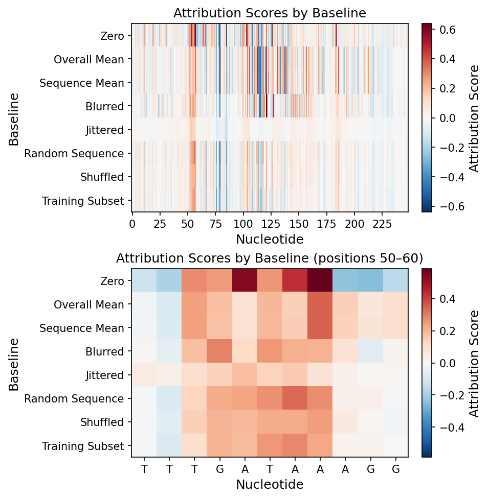Figure 8: Attribution scores for a single sequence across all baselines. Nucleotide positions 50–60 show consistently high attributions.

The attributions are relatively consistent across the baselines. As seen in Figure 8, nucleotide positions 50-60 have high attributions across all baselines. The positions with the high attributions correspond to the subsequence TGATAA. As we will see in the section on Motif Analysis, GATA has been shown to be an important enhancer motif in previous literature (de Almeida et al., 2022). The jittered baseline leads to faint attributions compared to the rest.

Note that even if the error ratio of all the attributions satisfies the threshold, there can still be qualitative differences between them. The completeness theorem only verifies that the sum of the attributions approximately matches the change in model predictions, but it does not verify that the distribution of the attributions across features is correct.

In Figure 9, you can see the attributions using the jittered baseline for the 200 sequences in the subset selected for attribution analysis sorted by the true enhancer activity.

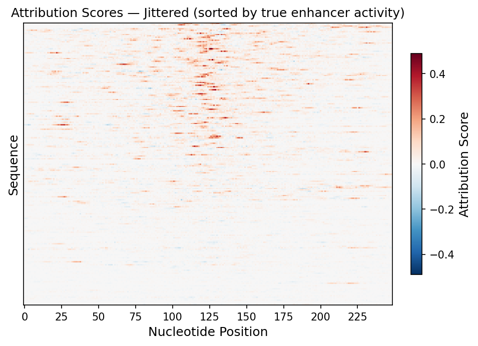Figure 9: Attribution scores using the jittered baseline for 200 sequences, sorted by true enhancer activity.

The attributions are more concentrated around the middle for the sequences with high enhancer activity (Figure 9). This can give us some confidence in the validity of the jittered baseline for identifying sequences with high enhancer activity because all enhancer sequences were centred around the part of the sequence with the highest regulatory activity (de Almeida et al., 2022).

The majority of attributions are positive. This is not surprising as we already saw in the section on Baseline Visualisations: all jittered embeddings lead to predictions lower than the mean and median predictions on the target sequences (see Figure 7).

Ablation Tests

We want to find out which of the baselines is the best at identifying the most influential nucleotides. For this, we use ablation tests. An ablation test means removing features in order of attribution to see whether the model predictions change in accordance with what the attributions indicate. More specifically, they work like this:

Ablation Test Process

1. Replace features in the order of attribution with a replacement embedding – an embedding that should “remove” the feature, similar to a baseline in integrated gradients
2. Record the model prediction at each ablation step
3. Calculate the signed Area Under Curve (AUC) under the curve of model predictions over the course of the ablations

When removing features with positive attributions from highest to lowest, a low AUC is better because ablating high attribution features should lead to steep drops in the predicted variable. When ablating features with negative attributions from lowest to highest, a high AUC is the best (Sturmfels et al., 2020).

Before calculating the AUC, we also min-max normalise the x axis for each of the sequences, so the axis represents the fraction of ablated nucleotides. This is so that sequences with more positive attributions do not automatically have a higher AUC just because there are more features to be ablated.

Importantly, we perform the ablation test on the intersection of converged sequences for all the baselines (because attributions without convergence are unreliable). It is necessary to do the ablations on the same sequences for each of the baselines due to selection bias: the AUC is strongly affected by the prediction at the unablated sequence. If some baselines only converge for sequences where the starting prediction is low, then they may have an advantage in the ablation tests when it comes to ablating positive attributions.

We note that ablation tests only reveal whether the rank of the attributions is correct, but they do not test the magnitude of attributions. This is because the magnitude of the change in model prediction upon ablation of a feature depends on the baseline used for ablation.

Notes on the Replacement Embedding

The replacement embedding we use for the ablations should be the same for every attribution baseline, so that the AUCs are comparable. This is because some replacement embeddings behave differently than others (as we have seen with the attribution baselines), so some may lead to much steeper drops over the course of ablation than others.

Additionally, the replacement embedding should not match any of the attribution baselines, otherwise it will result in circular reasoning. Integrated gradients shows how much a specific feature contributes to the prediction as the sequence moves from baseline to input. Hence, it is likely that, when replacing the feature by the attribution baseline, the prediction will change according to the attribution. While non-linear feature interactions mean single-feature ablation does not necessarily mirror integrated gradients’ simultaneous interpolation, using identical baselines can still bias the evaluation. So, when using the same embedding as an attribution baseline and a replacement embedding during ablation, an ablation test would be more of a confirmation that the attributions are calculated correctly rather than an estimate of how good the attributions are.

We used the random sequence baseline as a replacement embedding because:

1. It is almost certainly not the same across runs, so we can use it on any baseline
2. We can take multiple samples per ablation, leading to a less biased assessment

We took 4 samples per ablation.

We also perform a sanity check: we calculate the median AUC when we ablate features in random order (which should always be worse than ablating in the order mandated by the attributions). In this procedure, we ablate the same number of tokens for each sequence as are ablated in the corresponding ordered ablation case. We do not ablate padding tokens.

Ablation Test Results

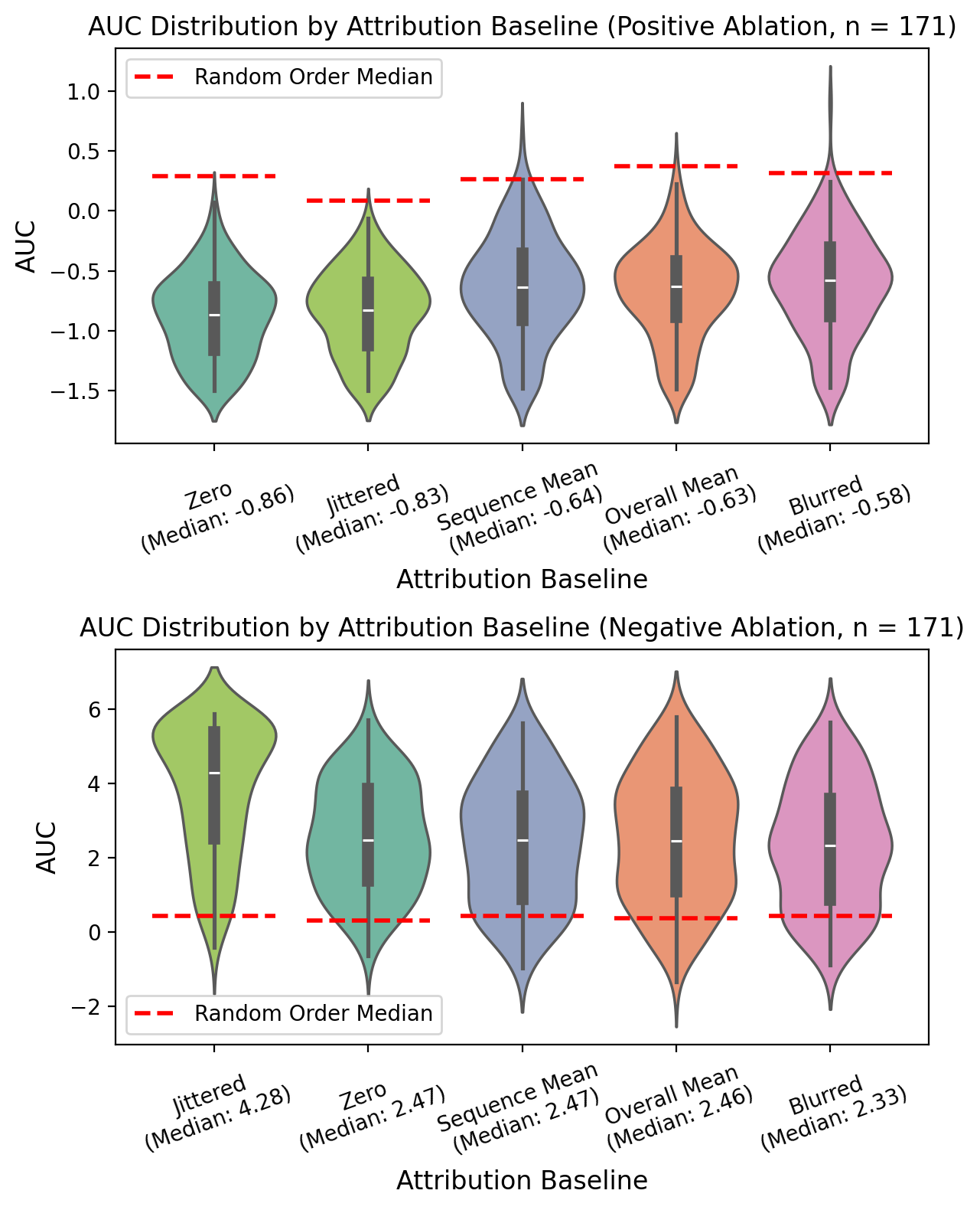Figure 10: Signed AUC distribution by attribution baseline for positive and negative ablation tests. The jittered and zero baselines perform best.

The intersection of converged sequences across these five baselines contains 171 sequences. As shown in Figure 10, the zero and jittered baselines perform best when ablating positively attributed nucleotides. The jittered baseline performs much better than the rest when ablating negatively attributed nucleotides. So, we will use the jittered baseline for the motif discovery.

For a randomly selected sequence, Figure 11 shows how the predictions evolve as we ablate nucleotides using the jittered baseline:

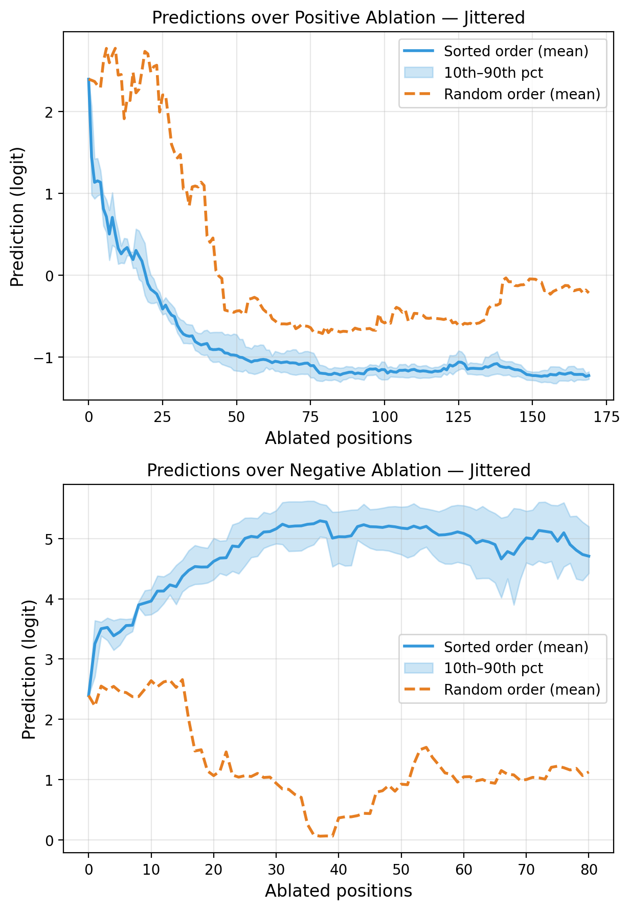Figure 11: Model predictions over the ablation of positively and negatively attributed features for a single sequence using the jittered baseline.

In the positive case there is a drop and, in the negative case, an increase in model predictions. In both cases, the AUCs are significantly better using the sorted order than the random order. Hence, this baseline seems to make reasonable attributions.

Motif Analysis

Having found the most promising baseline for attribution analysis, we calculate the attributions on the entire test set. We then extract motifs from these attributions by looking at whether some subsequences consistently have high or low attributions. For this, we use the TF-MoDISco algorithm.

TF-MoDISco

TF-MoDISco is an algorithm for motif discovery using importance scores from ML models (Shrikumar et al., 2018). We use the attributions we calculated as importance scores. These scores help the algorithm identify “seqlets,” which are short segments of the input sequence that significantly contribute to the model’s output. Once these important segments are found, TF-MoDISco groups them into broad “metaclusters” based on their shared activity patterns. Within each metacluster, it calculates the similarities between individual seqlets and clusters them together into aggregated motifs. Finally, the algorithm post-processes these groups by trimming weak boundaries and merging redundant patterns, ultimately producing a non-redundant set of predictive motifs learned by the network. It also outputs the “contribution” of each nucleotide in the motif. The contribution is the average importance score (here, the average attribution) for each nucleotide at the position within the motif.

Typically, TF-MoDISco also expects “hypothetical importance scores” as input. These scores estimate the potential importance of alternative nucleotides — that is, the bases not present at a given position in the sequence. Because we did not calculate or approximate these hypothetical scores, we assigned a value of zero to all non-occurring nucleotides. Consequently, the algorithm lacks the contextual information that tells it which nucleotide substitutions are functionally acceptable. Without this tolerance for minor variations, TF-MoDISco has a harder time merging highly similar motifs into a single consensus pattern, and may instead artificially fragment them into separate motifs.

Motifs

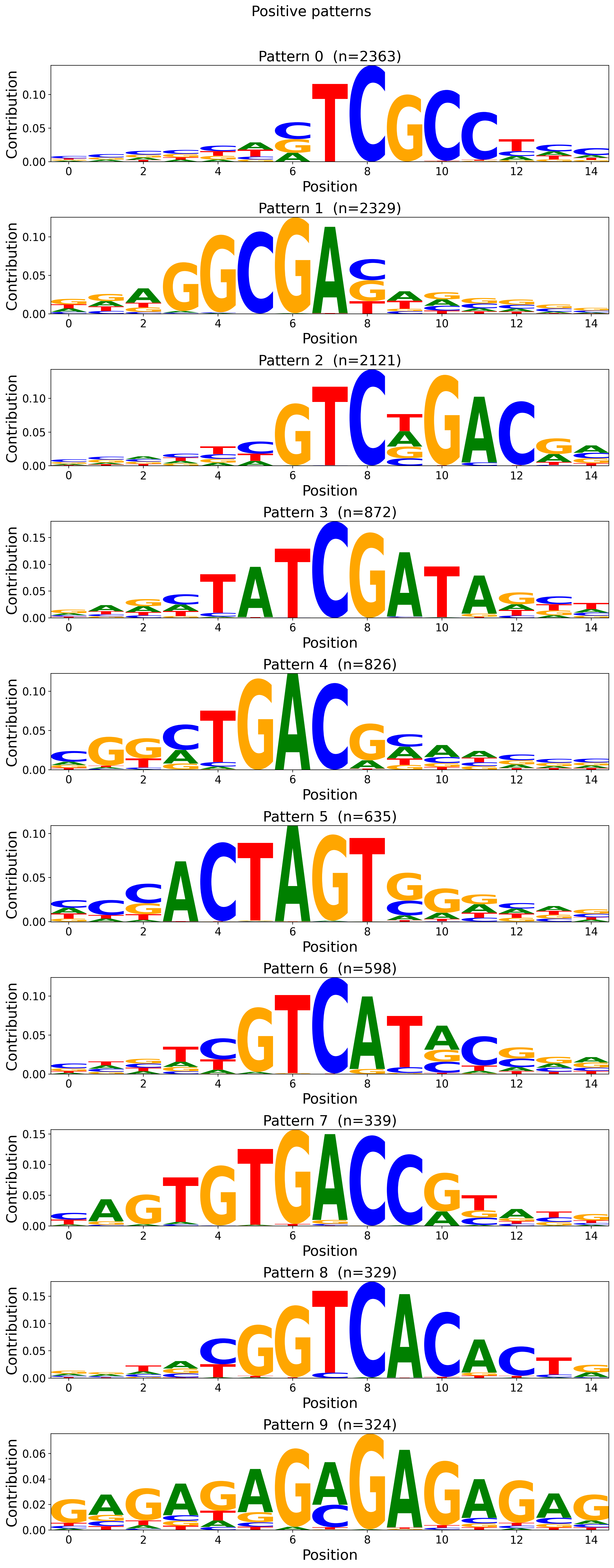
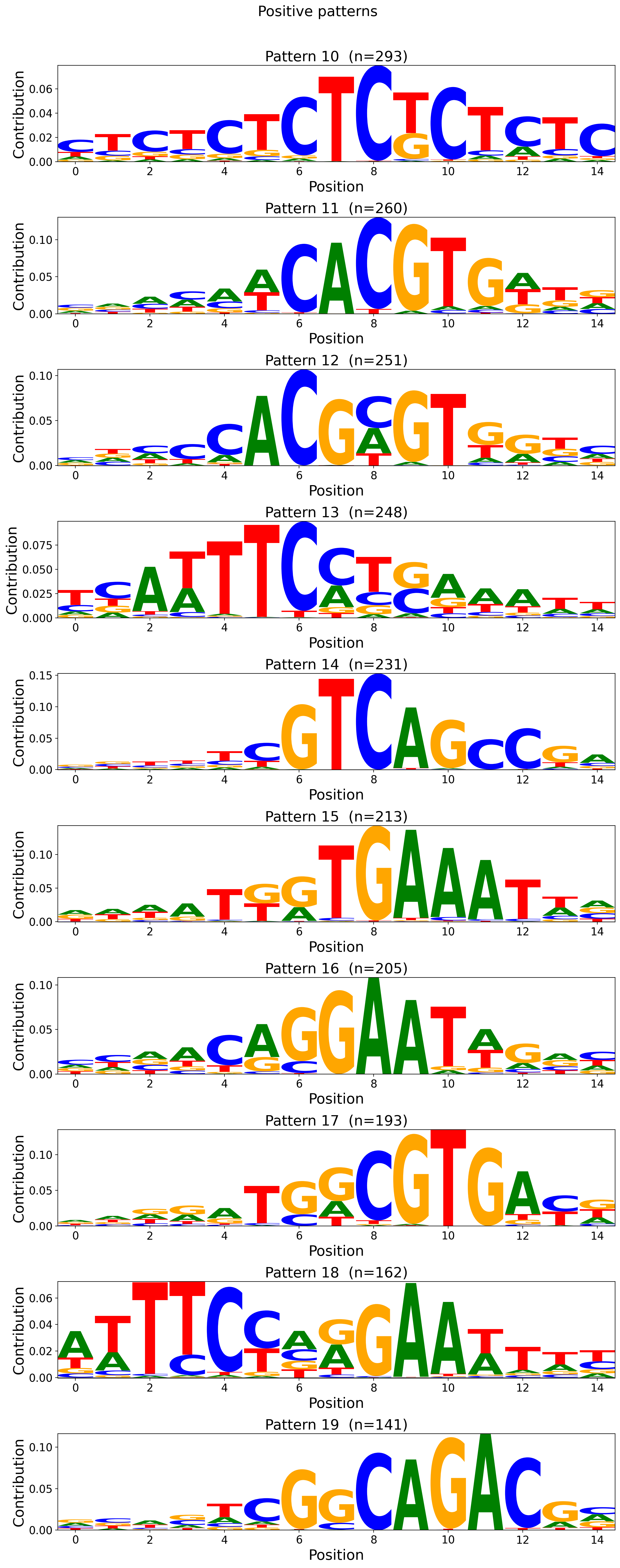
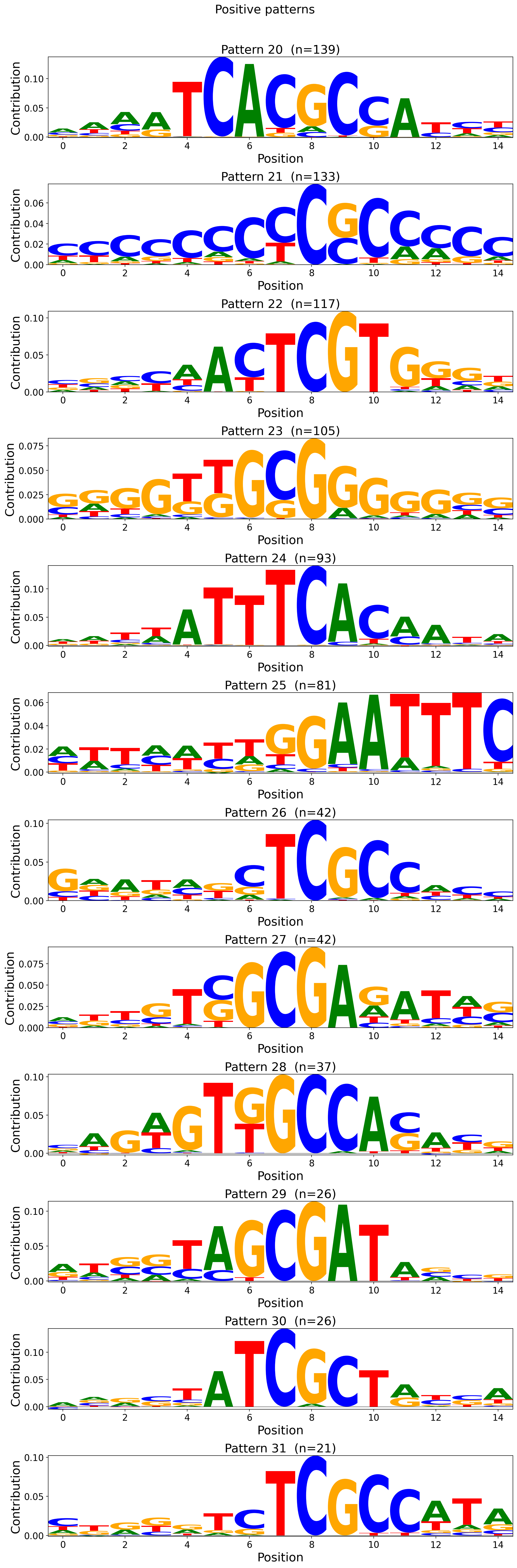
We show the TF-MoDISco patterns discovered by using the attributions generated using the jittered baseline. These attributions converged for 30,622 out of the 41,186 sequences (~74%). We did the motif analysis only on converged sequences. See Appendix D for the hyperparameters we used for TF-MoDISco. They mirror the hyperparameters used in DeepSTARR (de Almeida et al., 2022). In the patterns we present, 15 nucleotides are always shown while only a subset of these 15 positions is significant. This is for visualisation purposes. Figure 12 shows the 5 most frequent positive patterns found by TF-MoDISco (out of 32 positive patterns):

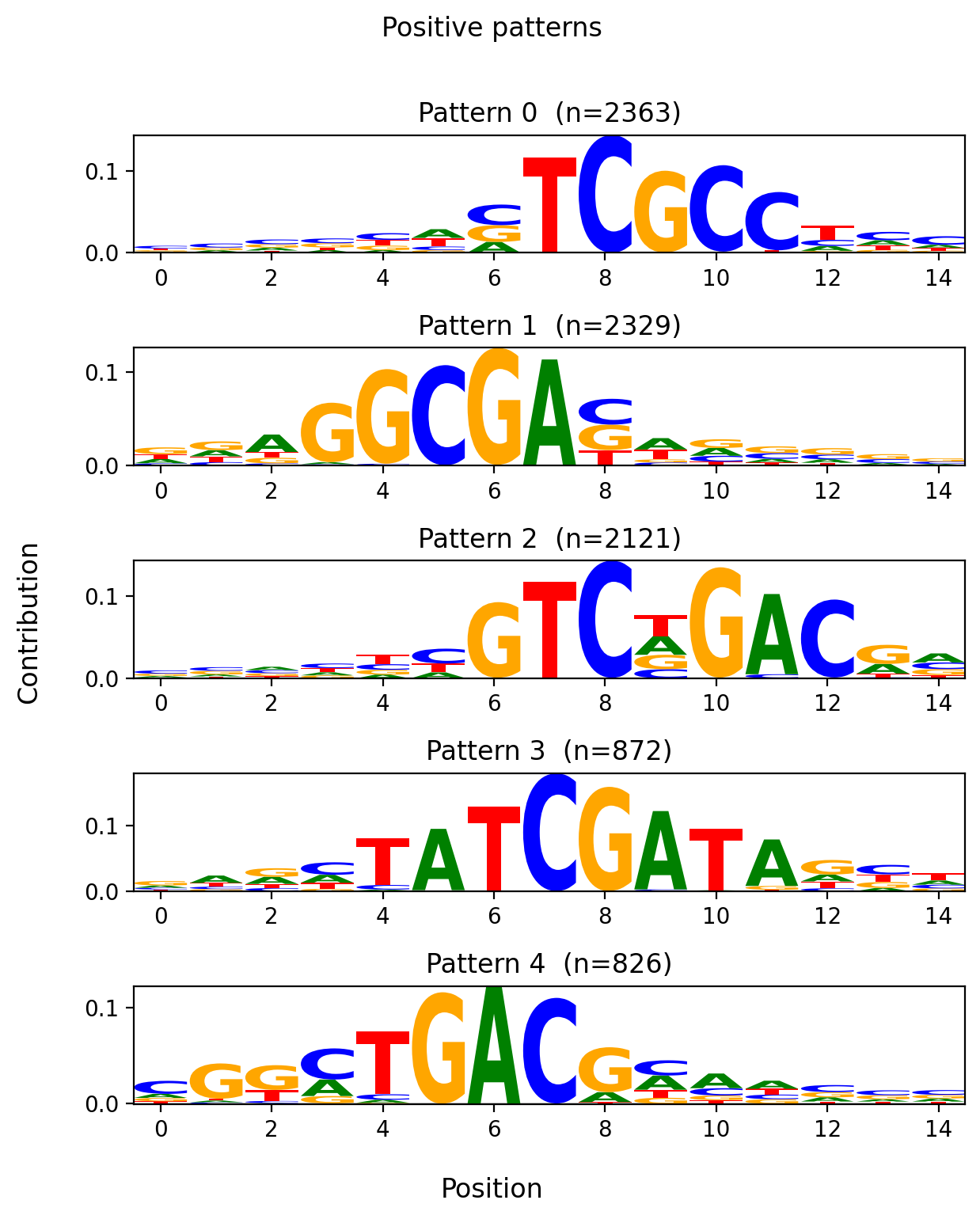Figure 12: Top 5 most frequent positive TF-MoDISco patterns from jittered baseline attributions.

The contribution is the average attribution for a nucleotide at its position, averaged across all the seqlets that were clustered to form the motif. The contribution of the important nucleotides is around 0.1, which means the model believes these nucleotides have a significant impact considering the model’s predictions range from -2 to 6 on the test set (see the section on Dataset and Training).

The 5 negative patterns found by TF-MoDISco are presented in Figure 13:

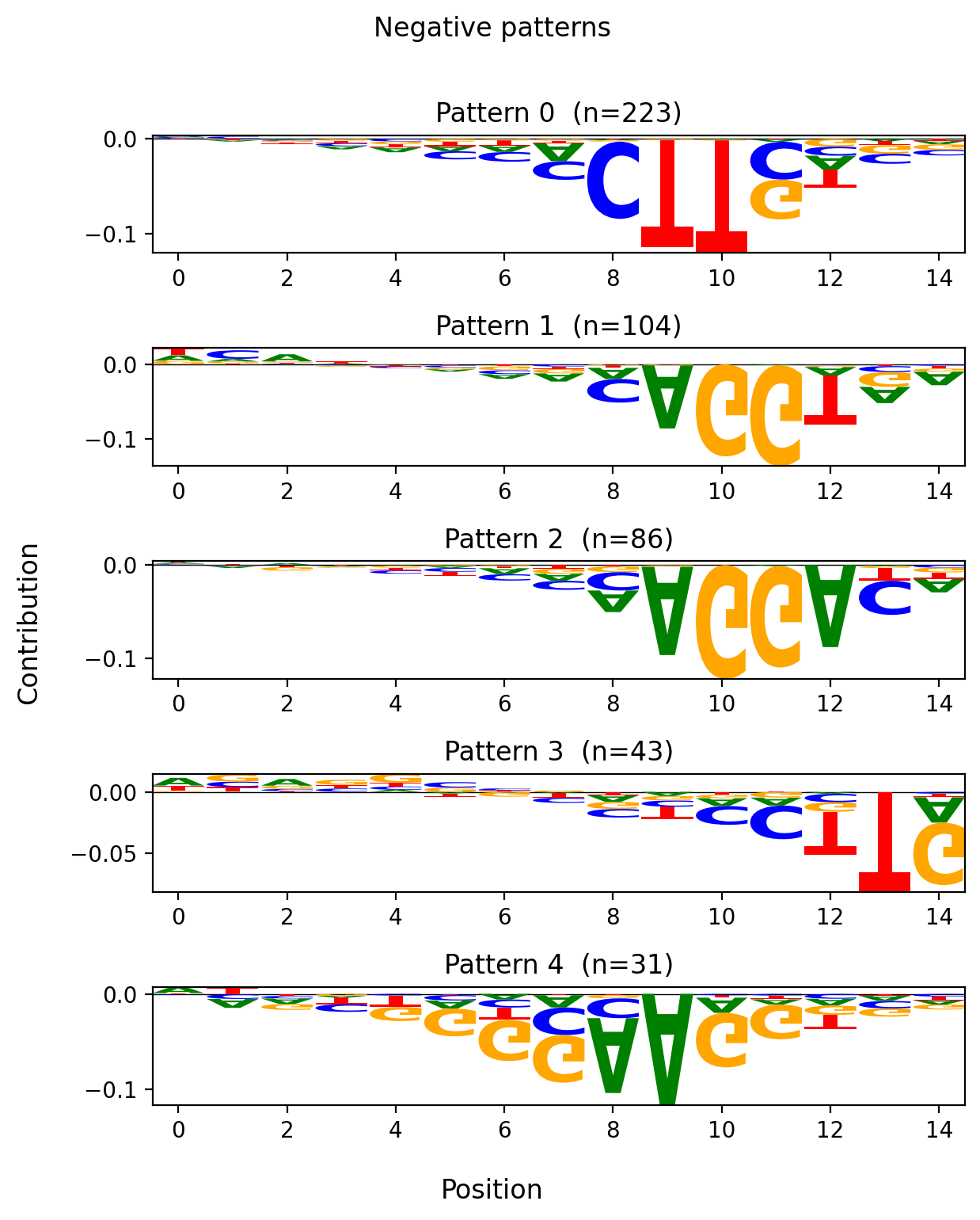Figure 13: Top 5 negative TF-MoDISco patterns. These occur less frequently than positive patterns, but have similar contribution magnitudes.

The negative patterns occur much less frequently than the positive patterns, but the magnitude of their contributions is similar. The negative patterns being rarer is not surprising given that we already saw in Figure 9 that the jittered baseline results in a majority of positive attributions. The rest of the motifs can be found in Appendix E.

Matching Found Motifs with Known Transcription Factor Binding Sites (TFBS)

We want to investigate whether the motifs we found using our attributions match TFBS already known in the literature. To achieve this, we match the motifs we found to the TFBS in the JASPAR database (Ovek Baydar et al., 2026). We used only the CORE collection of validated TFBS filtered by Drosophila melanogaster. For each TFBS, we only used the latest version, which filtered it down from 357 to 296 sites.

The matching algorithm works like this: for each TF-MoDISco motif we found, we match it with the JASPAR site whose position probability matrix (PPM), a matrix showing the probability of seeing each nucleotide at each position of a site, is most highly correlated with the PPM of the given TF-MoDISco motif. Before calculating the correlation, we weight the probabilities by the information content of the nucleotide probability distribution at each position to reduce the impact of uninformative positions (i.e. positions where each nucleotide is equally likely to occur, so the correlation would be high for these positions). We use the Pearson correlation. We then visualise the matches by plotting the sequence logos of the found motifs and those in JASPAR side by side.

In the visualised sequence logos, the y-axis represents information content measured in bits, calculated from the PPM at each position. The overall height of a column indicates the degree of sequence conservation at that position. Given the four possible DNA nucleotides, the maximum information content is 2 bits, denoting a perfectly conserved position where only a single nucleotide occurs. Conversely, a height of zero bits denotes a completely uninformative position where all four nucleotides appear with equal probability. Within each column, the height of an individual letter is proportional to the relative frequency of that specific nucleotide in the aligned sequences.

A selection of the matches for positive patterns appears in Figure 14 (our patterns are on the left while the known TFBS are on the right):
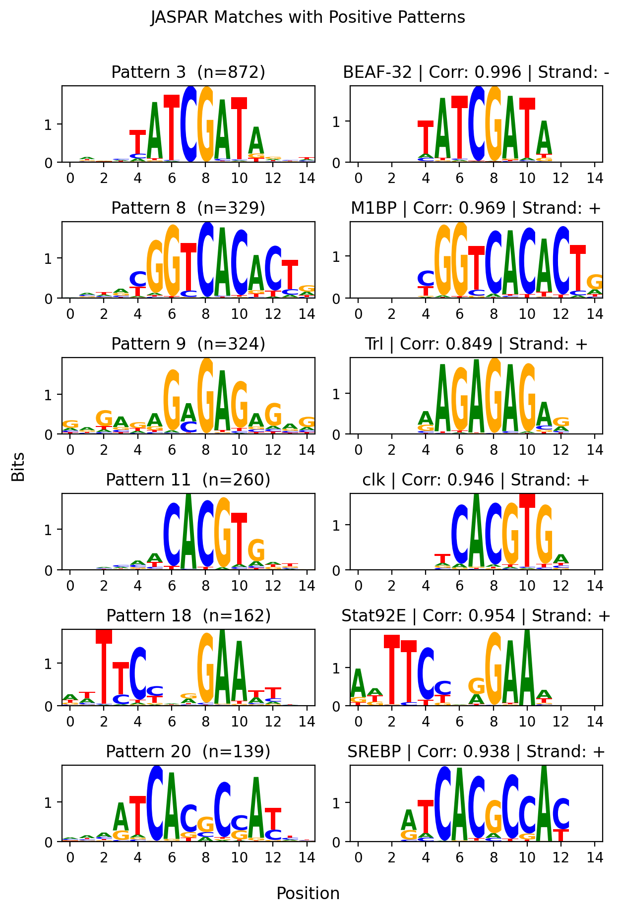Figure 14: Selected matches between positive TF-MoDISco patterns (left) and known JASPAR transcription factor binding sites (right).

Looking at Figure 14 and the FlyBase database, we can see that the transcription factors binding to these matched sites (with the exception of the insulator BEAF-32) act as activators (The FlyBase Consortium, 2002). This means these sequences function as enhancer sites that drive up gene expression. Consequently, the model has successfully recognised biologically important enhancer motifs.

DeepSTARR also mentions some known enhancer motifs (see Appendix F) (de Almeida et al., 2022). The motifs found by TF-MoDISco match some of them:

• Pattern 3 contains part of the GATA motif
• Pattern 9 is the GAGA-repeat

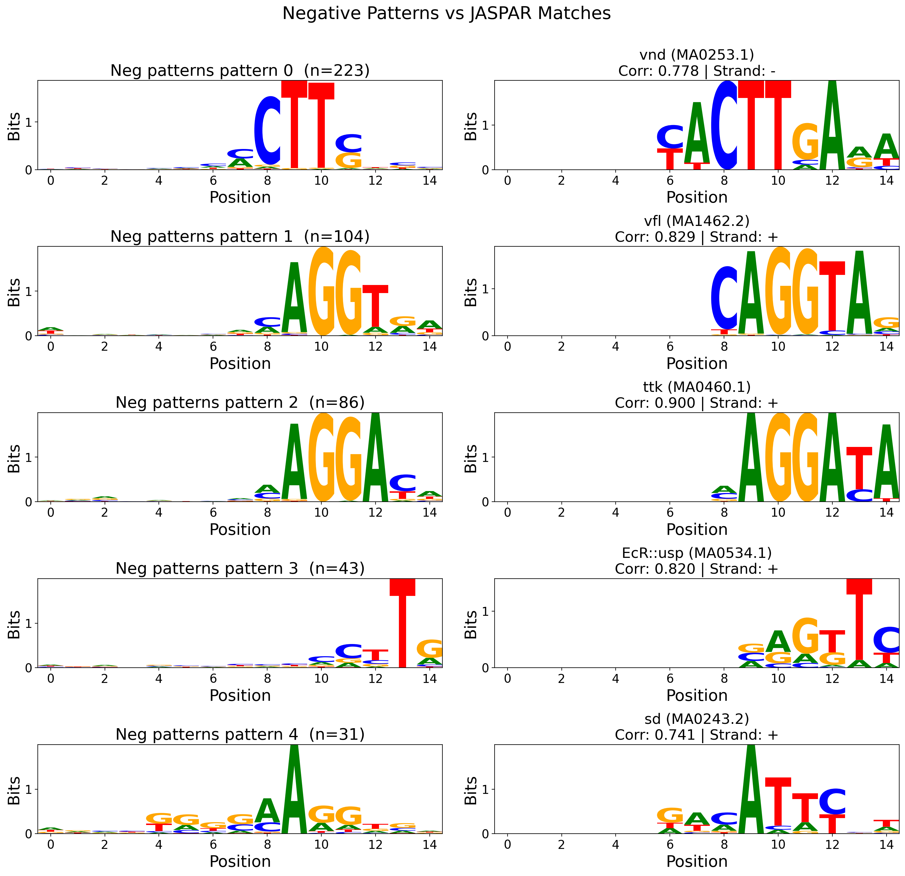
The equivalent plot for some of the negative patterns is in Figure 15:

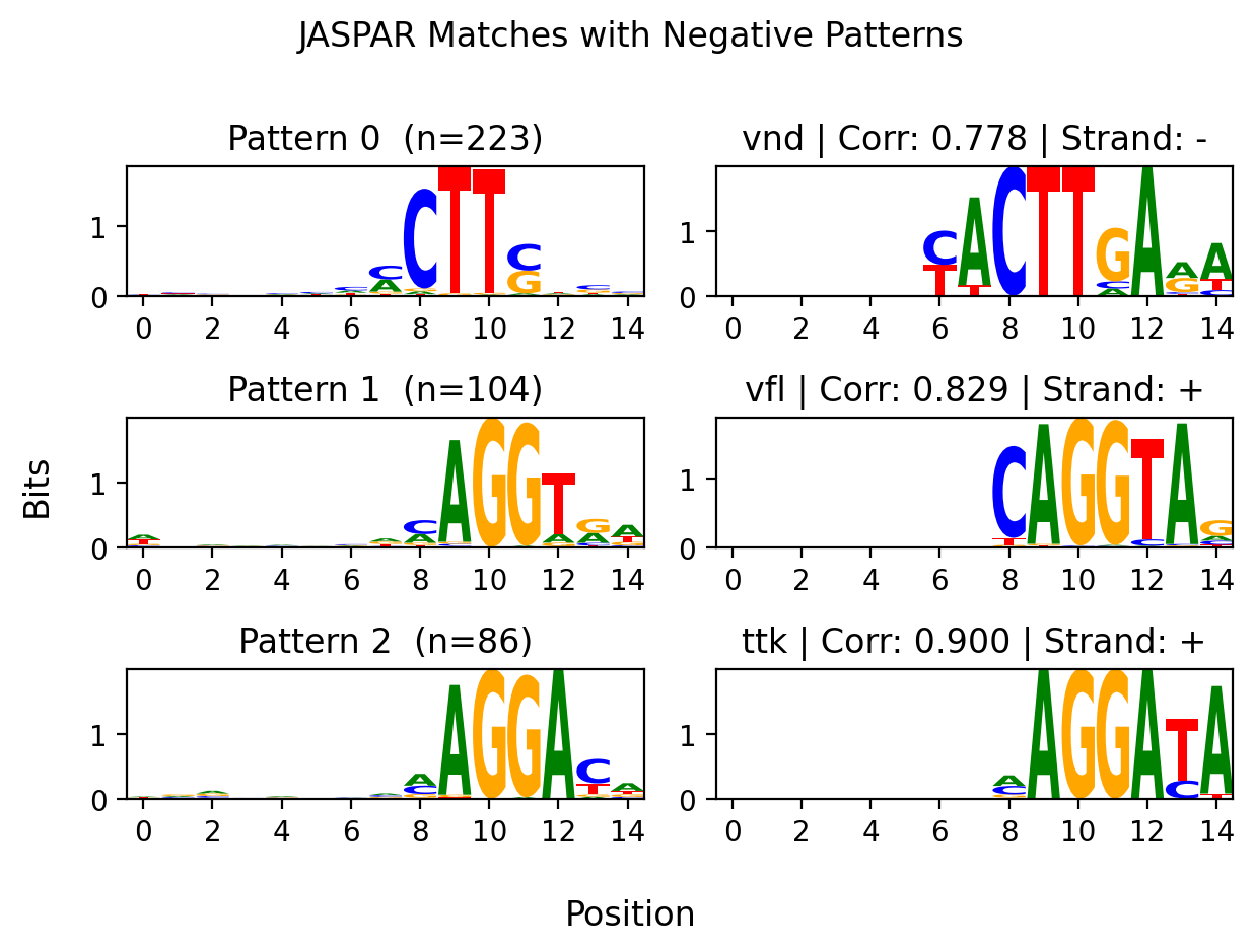Figure 15: Selected matches between negative TF-MoDISco patterns (left) and known JASPAR transcription factor binding sites (right).

Looking at Figure 15 and FlyBase reveals that, of the transcription factors associated with the matched binding sites above, only ttk is a repressor. vfl is an activator while vnd can act as either one depending on the context (The FlyBase Consortium, 2002). Concerning vfl, it should be mentioned the binding site is very similar to another binding site called esg, which is a repressor (Ovek Baydar et al., 2026). Hence, the model did recognise a binding site for a repressor in ttk, but the rest of the results are more ambiguous.

The JASPAR matches for all patterns can be found in Appendix G. In this section, we showed only the clearest matches – many of the matches found by the algorithm do not look like genuine matches because the magnitudes of the information content do not match. This is likely because the Pearson correlation only looks at linear relationships and does not consider whether the magnitudes of the variables match.

Limitations

While our workflow provides a practical method for interpreting genomic foundation models, several limitations remain regarding both the methodology and the biological context. Integrated gradients assumes a continuous, smooth feature space; when applied to categorical data like DNA, this interpolation traverses regions of the embedding space that do not correspond to any nucleotide sequence. In this embedding space, the model’s gradients can become arbitrary, leading to noisy attributions (Majdandzic et al., 2023).

The baseline’s default prediction level skews the direction of the resulting attributions. As we observed, understanding the distribution of the model’s predictions at a given baseline is necessary to understand these results. Because our chosen jittered baseline yielded lower average predictions (see Figure 7), the resulting attributions were predominantly positive to bridge that gap (see Figure 9).

There is an unresolved trade-off between using fixed baselines (like in integrated gradients) versus sampling based baselines (as in expected gradients). Fixed baselines, like the zero or overall mean embedding, produce the same prediction regardless of the target sequence, which makes attribution results across different sequences more directly comparable. However, our ablation tests showed that a sampling based baseline, the jittered baseline, performed best (see Figure 10) despite the risk of feeding the model out-of-distribution noise.

Additionally, our motif discovery was constrained; because we did not compute hypothetical attributions, TF-MoDISco may have lacked the context needed to seamlessly merge similar motifs into unified consensus patterns.

Finally, because none of the motifs we found were tested in the lab, we do not know if motifs that were not matched with known transcription factor binding sites are valid or simply noise. Further, we did not analyse in detail the motifs that are not well-matched with known motifs to check whether there may be some biological significance to them.

Conclusion

This study outlines a practical pipeline for performing attribution analysis on genomic foundation models using integrated gradients. Because adapting interpretability methods to categorical DNA data is not straightforward, our primary goal was to demonstrate how to approach this process. We emphasise the steps required for success: defining what a baseline means in a genomic context, verifying attribution validity through convergence checks, and evaluating the best baseline choice via ablation tests.

The attributions generated via our jittered baseline guided TF-MoDISco to recover established Drosophila regulatory motifs. Finding these well-known motifs validates that our pipeline successfully uncovers genuine biological grammar learned by the model. However, our motif analysis serves primarily as a proof-of-concept rather than an exhaustive biological study. The exploration of these patterns is not extensive, and deeper investigation is needed to fully characterise the specific motifs and potentially spurious signals the model leverages.

Ultimately, we hope this rigorous approach to baseline selection and validation provides a reliable blueprint for practitioners seeking to interrogate what their genomic foundation models have learned.

Takeaways

Pipeline for Integrated/Expected Gradients

• Check the distribution of embedding values for all the baselines and compare them against embedding values of the original sequences – anything too far out of distribution could be a problem.
• Compare distribution of predictions at baselines to the predictions on the original sequences – this reveals whether the baselines are biased towards lower or higher predictions than the original sequences, which can affect attributions down the line.
• Check the convergence of the attributions on a subset of the data at different numbers of integration steps – this will help select the right number of integration steps for each baseline, so they converge for most sequences. This ensures the sum of the attributions correctly accounts for the difference in predictions at the baseline and the target sequence.
• Conduct ablation tests to find the most promising baseline. Use a replacement embedding that does not match the attribution baselines to avoid circular reasoning. Use the same replacement embedding for the evaluation of all attribution baselines, so the signed AUCs are comparable across sequences.

Key Results

• Sampling-based baselines can outperform fixed baselines: While fixed baselines (like the zero or overall mean embedding) offer stable baseline predictions, ablation tests revealed that a sampling-based baseline (Gaussian jitter) was the most effective at accurately identifying the most influential nucleotides.
• Attributions reveal true biological grammar: Clustering the sequence-level attributions from the best-performing baseline (via TF-MoDISco) successfully recovers known, experimentally validated transcription factor binding sites found in the JASPAR database. This confirms that the genomic foundation model’s predictions are partially driven by biological rules.

Thank You Note

I want to thank my supervisors Mafalda Ribeiro and Jonas Hirsch at InstaDeep, who co-wrote this article with me, gave invaluable feedback on it even after my internship had ended, and from whom I learned so much about software engineering, machine learning, and biology.

Disclaimer

This is my personal interpretation of the work done as part of my internship at InstaDeep. All data are open source. All findings and claims are taken from the cited papers or public sources. No confidential information from my time at InstaDeep has been used in this article.

References

Anthropic. (2025, July). Circuits Update—July 2025. https://transformer-circuits.pub/2025/july-update/index.html

Boshar, S., Evans, B., Tang, Z., Picard, A., Adel, Y., Lorbeer, F. K., Rajesh, C., Karch, T., Sidbon, S., Emms, D., Mendoza-Revilla, J., Al-Ani, F., Seitz, E., Schiff, Y., Bornachot, Y., Hernandez, A., Lopez, M., Laterre, A., Beguir, K., … Pierrot, T. (2025). A foundational model for joint sequence-function multi-species modeling at scale for long-range genomic prediction. bioRxiv. https://doi.org/10.64898/2025.12.22.695963

Consens, M. E., Dufault, C., Wainberg, M., Forster, D., Karimzadeh, M., Goodarzi, H., Theis, F. J., Moses, A., & Wang, B. (2025). Transformers and genome language models. Nature Machine Intelligence, 7(3), 346–362. https://doi.org/10.1038/s42256-025-01007-9

The FlyBase Consortium (2002). The FlyBase database of the Drosophila genome projects and community literature. Nucleic Acids Research, 30(1), 106–108. https://doi.org/10.1093/nar/30.1.106

de Almeida, B. P., Reiter, F., Pagani, M., & Stark, A. (2022). DeepSTARR predicts enhancer activity from DNA sequence and enables the de novo design of synthetic enhancers. Nature Genetics, 54(5), 613–624. https://doi.org/10.1038/s41588-022-01048-5

Erion, G., Janizek, J. D., Sturmfels, P., Lundberg, S., & Lee, S.-I. (2020). Improving performance of deep learning models with axiomatic attribution priors and expected gradients. https://arxiv.org/abs/1906.10670

InstaDeep. (2026). NTv3 benchmark. https://huggingface.co/spaces/InstaDeepAI/ntv3_benchmark

Libbrecht, M. W., & Noble, W. S. (2015). Machine learning applications in genetics and genomics. Nature Reviews Genetics, 16(6), 321–332. https://doi.org/10.1038/nrg3920

Majdandzic, A., Rajesh, C., & Koo, P. K. (2023). Correcting gradient-based interpretations of deep neural networks for genomics. Genome Biology, 24(1), 109. https://doi.org/10.1186/s13059-023-02956-3

Ovek Baydar, D., Rauluseviciute, I., Aronsen, D. R., Blanc-Mathieu, R., Bonthuis, I., de Beukelaer, H., Ferenc, K., Jegou, A., Kumar, V., Lemma, R. B., Lucas, J., Pochon, M., Yun, C. M., Ramalingam, V., Deshpande, S. S., Patel, A., Marinov, G. K., Wang, A. T., Aguirre, A., … Mathelier, A. (2026). JASPAR 2026: Expansion of transcription factor binding profiles and integration of deep learning models. Nucleic Acids Research, 54(D1), D184–D193. https://doi.org/10.1093/nar/gkaf1209

Shrikumar, A., Tian, K., Shcherbina, A., Avsec, Z., Banerjee, A., Sharmin, M., Nair, S., & Kundaje, A. (2018). TF-MoDISco v0.4.4.2-alpha: Technical Note. CoRR, abs/1811.00416. http://arxiv.org/abs/1811.00416

Shu, L., Tang, J., Guan, X., & Zhang, D. (2026). A comprehensive survey of genome language models in bioinformatics. Briefings in Bioinformatics, 27(1), bbaf724. https://doi.org/10.1093/bib/bbaf724

Simonyan, K., Vedaldi, A., & Zisserman, A. (2014). Deep Inside Convolutional Networks: Visualising Image Classification Models and Saliency Maps. https://arxiv.org/abs/1312.6034

Sturmfels, P., Lundberg, S., & Lee, S.-I. (2020). Visualizing the Impact of Feature Attribution Baselines. Distill. https://doi.org/10.23915/distill.00022

Sundararajan, M., Taly, A., & Yan, Q. (2017). Axiomatic Attribution for Deep Networks. In D. Precup & Y. W. Teh (Eds.), Proceedings of the 34th International Conference on Machine Learning (Vol. 70, pp. 3319–3328). PMLR. https://proceedings.mlr.press/v70/sundararajan17a.html

Xu, S., Venugopalan, S., & Sundararajan, M. (2020, June). Attribution in Scale and Space. Proceedings of the IEEE/CVF Conference on Computer Vision and Pattern Recognition (CVPR).

Appendices

Appendix A: Fine-tuning Hyperparameters

Training Epochs	3
Learning Rate	5e-4
Batch Size	32
Warmup Steps	500
Linear Learning Rate Weight Decay	0.01

Appendix B: Predictions Across Interpolation

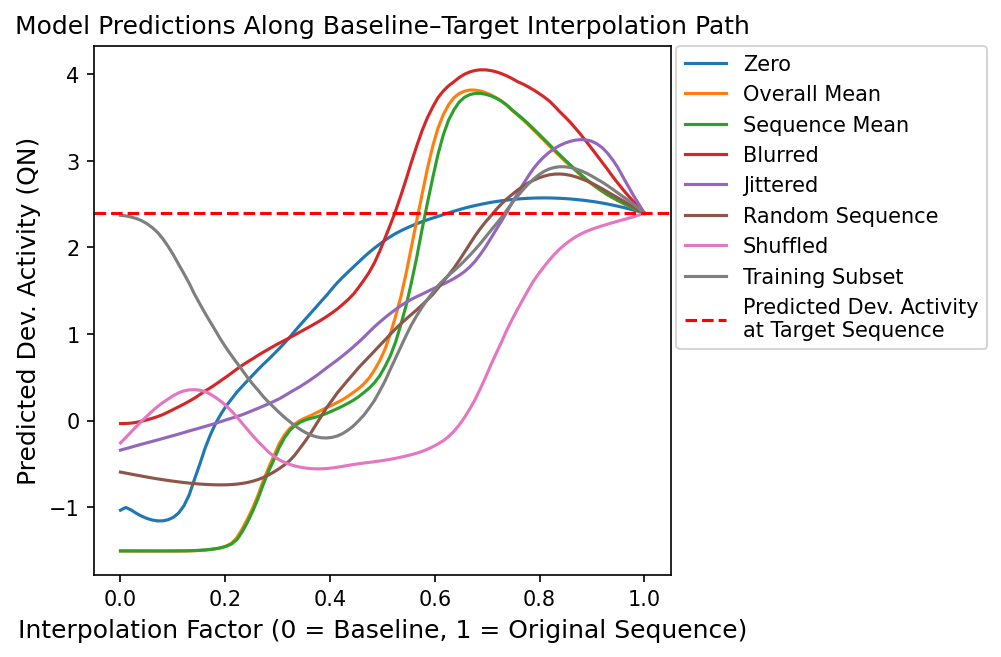Figure B1: Model predictions along the interpolation path from baseline to target sequence for each baseline.

The model’s prediction landscape between the baselines and the real sequences is highly non-linear and dependent on the baseline.

Appendix C: Convergence Analysis

To get an idea of how many integration steps are necessary for each baseline, we choose ten sequences at random from the set of sequences selected for attribution and measure the mean error ratio at different numbers of integration steps.

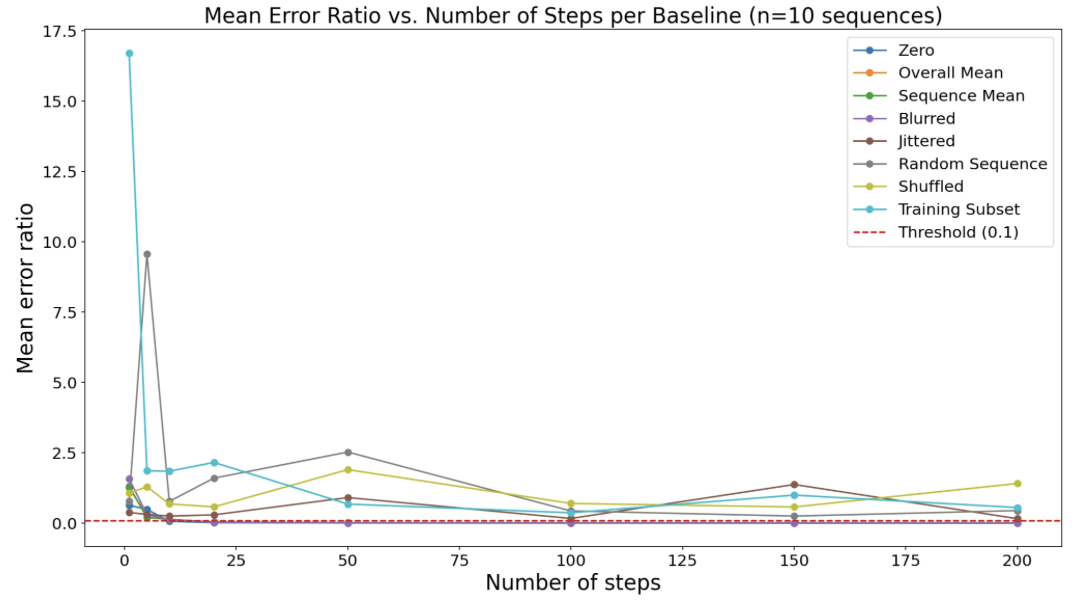Figure C1: Error ratio $\epsilon$ over different numbers of integration steps.

At 200 integration steps, the jittered, random sequence, shuffled, and training subset baselines exceed the error ratio threshold.

Given this, we choose the following numbers of steps for the baselines (the expected gradients baselines are in italic):

Baseline	Number of Integration Steps
Zero	200
Overall Mean	200
Sequence Mean	200
Blurred	300
Jittered	1,000
Random Sequence	1,000
Shuffled	1,000
Training Subset	1,000

With these steps, we calculate the attributions on the 200 sequences selected for attribution calculation and report the share of sequences meeting the convergence criterion.

Baseline	Fraction of Sequences Below Error Ratio Threshold
Zero	99.5%
Overall Mean	99.5%
Sequence Mean	100.0%
Blurred	99.5%
Jittered	86.5%
Random Sequence	73.0%
Shuffled	72.0%
Training Subset	58.5%

Appendix D: TF-MoDISco Hyperparameters

Sliding Window Size	15
Flank Size	5
Maximum Seqlets per Metacluster	50,000
Target Seqlet FDR	0.2
Minimum Metacluster Size	100
Trim to Window Size	15
Initial Flank to Add	5

Appendix E: Motifs

Positive TF-MoDISco patterns 0–9.

Positive TF-MoDISco patterns 10–19.

Positive TF-MoDISco patterns 20–31.

Negative TF-MoDISco patterns 0-4.

Appendix F: Enhancer Motifs from DeepSTARR

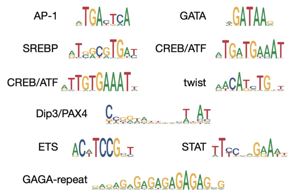Enhancer motifs from the DeepSTARR paper (de Almeida et al., 2022).

Appendix G: JASPAR Motif Matches

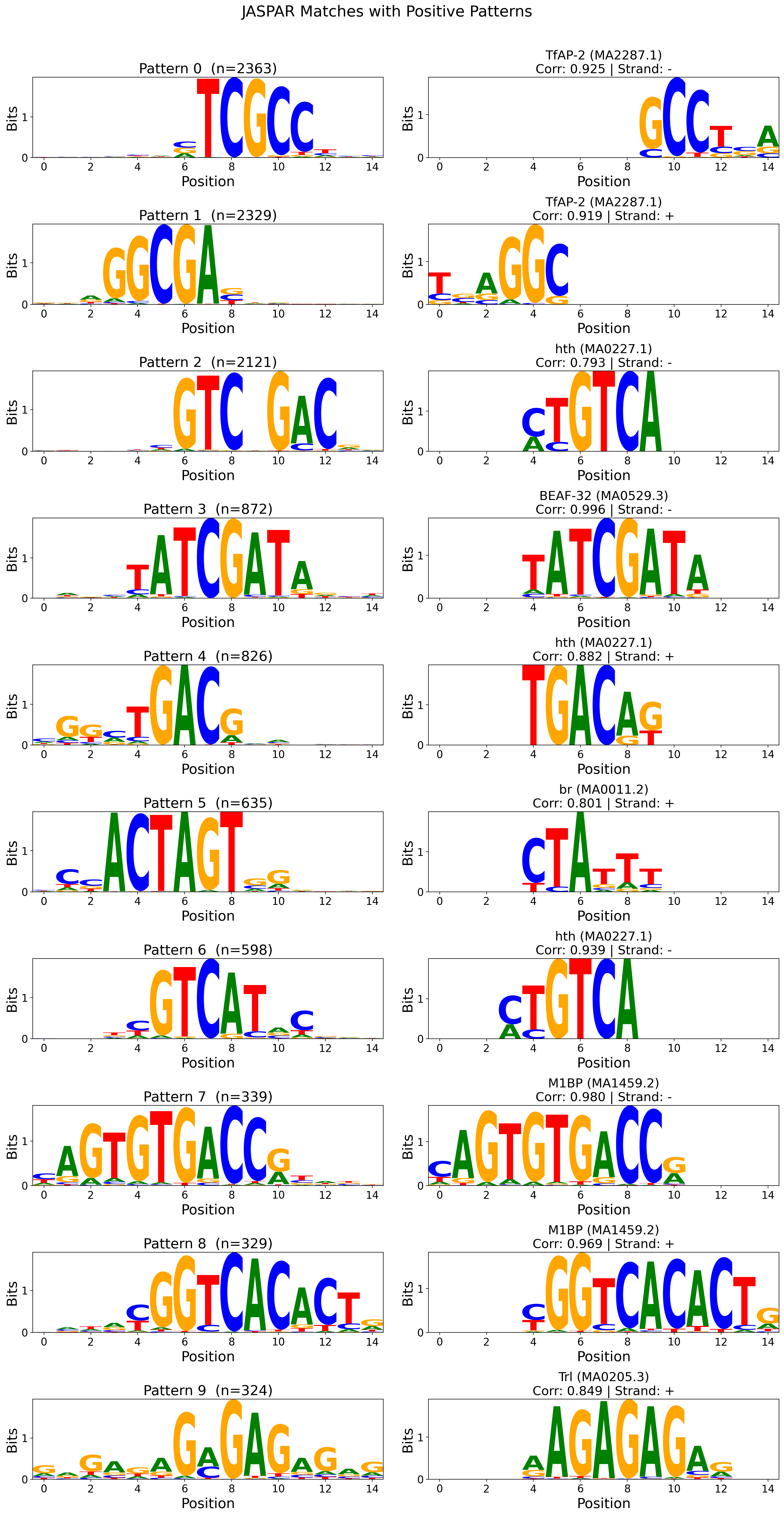JASPAR motif matches for positive patterns 0–9.

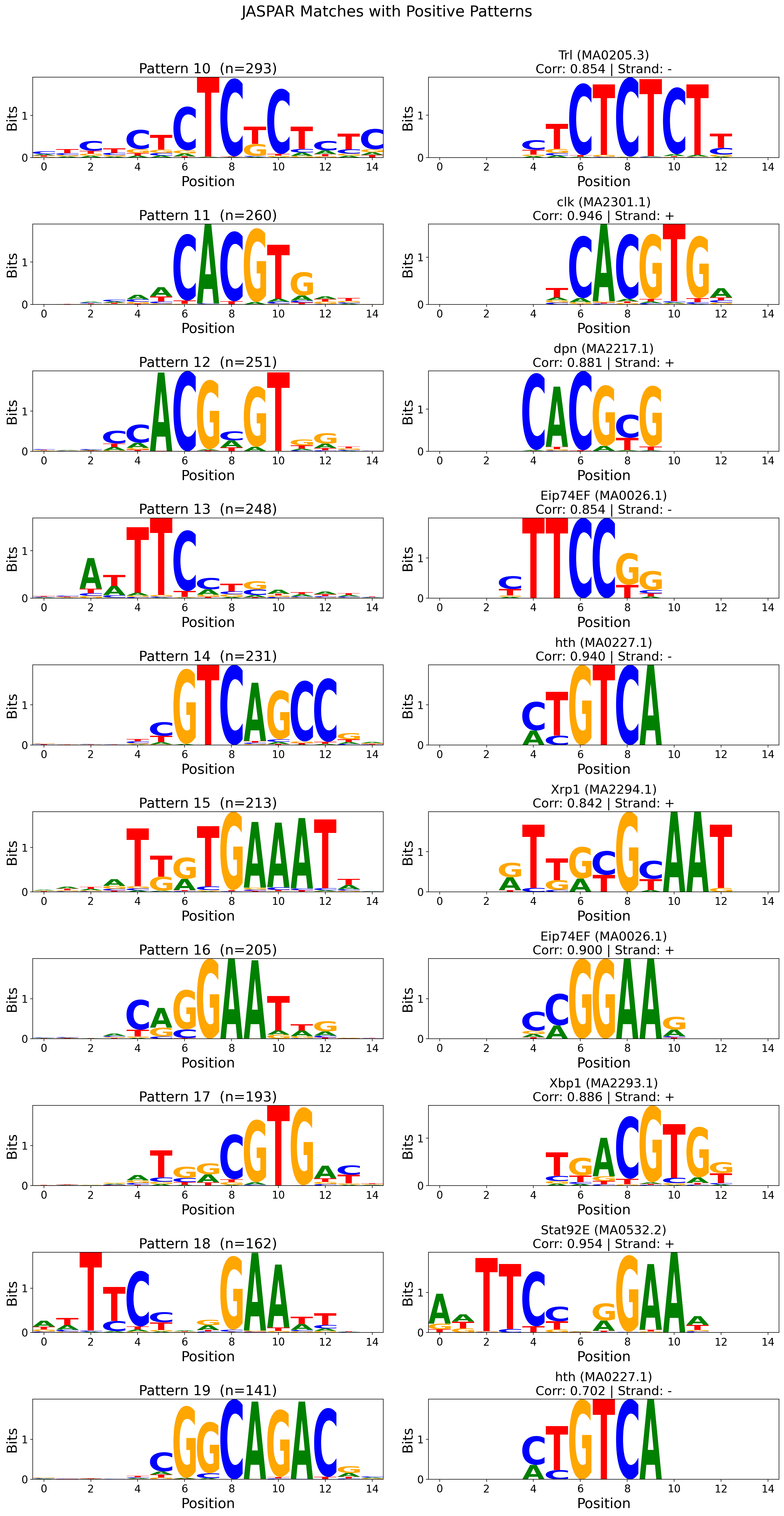JASPAR motif matches for positive patterns 10–19.

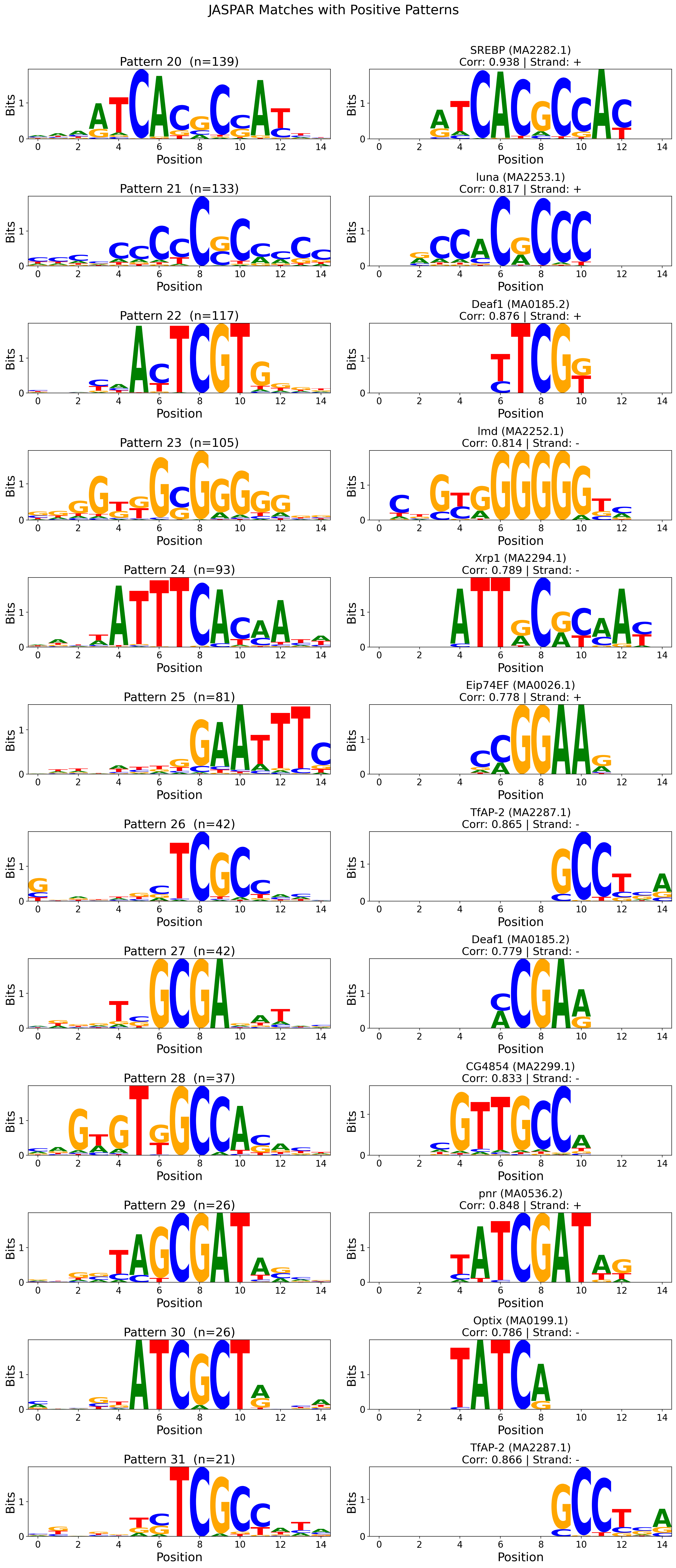JASPAR motif matches for positive patterns 20–31.

JASPAR motif matches for all negative patterns.